An introduction to Reinforcement learning

Reinforcement Learning
1. What is Reinforcement Learning?
Reinforcement learning is a machine learning training method based on rewarding desired behaviors and punishing undesired ones.
In general, a reinforcement learning agent – the entity being trained – is able to perceive and interpret its environment, take actions and learn through trial and error.
Key Features of Reinforcement Learning:
- The agent is not instructed about the environment and what actions need to be taken. It takes the next action and changes states according to the feedback of the previous action.
- RL based on the trial and error process.
- Feedback is always delayed, not instantaneous. Many real-world problems have long time horizons where the consequences of actions may not be seen for hours, days or even longer. This is in contrast to supervised learning, where feedback is instantaneous.
- The environment is stochastic, and the agent needs to explore it to reach to get the maximum positive rewards.
2. Usecases and challenges of Reinforcement Learning?
- Here are some reasons for using Reinforcement Learning:
- Helps to find best possible action to take in a specific situation.
- Helps to discover which action gains the highest reward over the longer period.
- Allows to figure out the best method for obtaining large rewards.
- Here are some conditions when should not use reinforcement learning model.
- When the problem is simple and can be solved with a simple rule-based approach.
- When we have enough data to solve the problem with a supervised learning method
- Reinforcement Learning is computing-heavy and time-consuming.
- Pros and Cons of Reinforcement Learning:
- Pros:
- RL is a powerful technique that can be used to solve complex problems.
- RL is a general-purpose technique that can be applied to any problem.
- It can be used to solve problems that are not well defined.
- …
- Cons:
- Reinforcement learning is a slow process.
- It requires a lot of data to train the model.
- It is difficult to debug the model.
- …
- Pros:
3. Reinforcement Learning vs Supervised Learning
| Parameters | Reinforcement Learning | Supervised Learning |
|---|---|---|
| Decision style | RL takes decisions sequentially. | Decision is made on the input given at the beginning. |
| Works on | Works on interacting with the environment. | Works on examples or given sample data. |
| Dependency on decision | In RL decision is dependent on the previous decision. | In supervised learning, the decision is independent of each other. |
| Best suited | Supports and work better where human interaction is prevalent. | It is mostly operated with an interactive software system or applications. |
| Example | Chess game AI, auto car,… | Classification, Regression,… |
4. Types of Reinforcement Learning
There are two types of reinforcement learning methods: positive and negative.
| Characteristic | Positive Reinforcement | Negative Reinforcement |
|---|---|---|
| Definition | Positive reinforcement involves rewarding the agent for taking specific actions or making certain decisions. When the agent performs a desirable action, it receives a positive reward, which encourages it to repeat the behavior in the future. | Negative reinforcement involves punishing the agent for undesirable actions or decisions. When the agent makes a suboptimal choice or takes a wrong action, it receives a negative reward, which discourages it from repeating that behavior. |
| Effect on behavior | Encourages the agent to repeat desired actions | Discourages the agent from repeating undesirable actions |
| Example | Teaching a dog to sit. We give the dog a positive reward when it sits which encourages it to continue sitting in the future | Think of a self-driving car as an agent. If the car takes a wrong turn or commits a traffic violation, it might receive a negative reward. This negative reward discourages the car from making such mistakes in the future. |
5. Terms used in Reinforcement Learning
- Agent: an entity that can be aware of and explore the maze environment, making decisions and taking actions to navigate through the maze.
- Example: In a maze game, the player controlling the character that moves through the maze is the agent.
- Environment (E): The maze itself, where the agent (player) is located and has to find a way out. In RL, the environment is stochastic, meaning the layout of the maze and any obstacles might change or have randomness.
- Example: The maze with its walls, pathways, and exit represents the environment in the maze game.
- Action (A): The set of all possible moves that the agent can make within the maze to navigate from its current position to another location in the maze.
- Example: In a maze game, the actions include moving up, down, left, and right to traverse the maze, or in some cases, taking no action (standing still).
- State (S): A situation returned by the environment after each action taken by the agent, representing the agent’s current position in the maze.
- Example: In a maze game, the state could be the specific coordinates (row and column) of the character within the maze, which indicates the character’s current location.
- Reward (R): Feedback returned to the agent (player) from the environment (maze) to evaluate the action taken by the player. It indicates how desirable or advantageous the player’s actions are.
- Example: In the maze game, the player might receive a positive reward for reaching the exit and successfully completing the maze, while receiving a negative reward for hitting a wall or making inefficient moves.
- Policy (π): A strategy applied by the agent (player) to decide the next action based on the current state (position in the maze). It’s a set of rules or heuristics used to determine the best move.
- Example: In the maze game, the player’s policy might be to always choose the direction that brings them closer to the exit, avoiding walls and dead ends.
- Value (V): The expected sum of all future rewards that the agent can achieve from a particular state while following a specific policy. It represents the long-term desirability of a state in terms of the cumulative rewards. Used to evaluate states and helps the agent make decisions about which states to prioritize or avoid based on their long-term desirability.
- Example: In the maze game, the value of a specific location within the maze represents how good or bad it is to be at that location, considering the expected future rewards, such as reaching the exit with fewer moves.
- Q value or action value (Q): It is mostly similar to the value, but it describes the value of taking an action a in state s under a policy π and then following a specific policy ‘π’ for the rest of the interaction with the environment. In other words, it quantifies how good it is to take a particular action in a given state under a given policy (which action to take in each state to maximize its long-term reward).
- Example: the Q value for a particular state-action pair represents the expected cumulative reward if the agent (player) chooses a specific action in a specific state and follows its policy. For instance, if the agent is in a state ‘S’ (position) and the available actions are ‘move left,’ ‘move right,’ ‘move up,’ and ‘move down,’ the Q values would be computed for each of these actions in that state. The Q values help the agent make informed decisions about which action to take in each state to maximize its long-term reward.
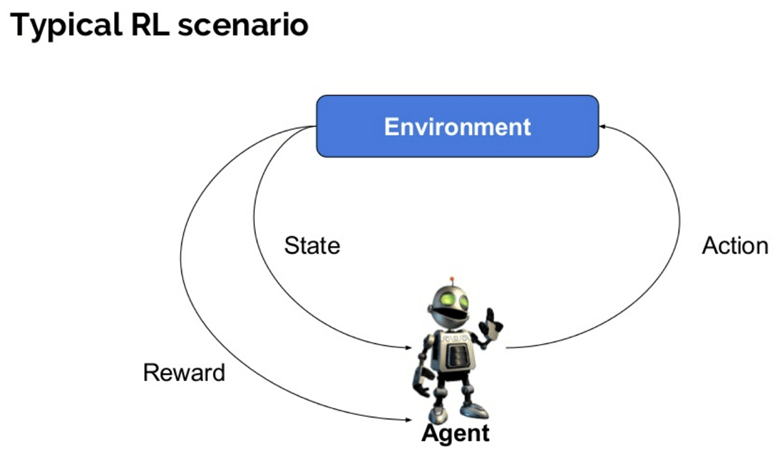
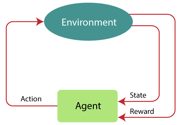
Typical RL Scenario
6. Approaches to implement Reinforcement Learning
6.1 Value-Based
- The value-based approach is about to find the optimal value function, which is the maximum value at a state under any policy.
- Therefore, the agent expects the long-term return at any state(s) under policy π.
6.2 Policy-based
In a policy-based RL method, you try to come up with such a policy that the action performed in every state helps you to gain maximum reward in the future.
Two types of policy-based methods are:
- Deterministic: For any state, the same action is produced by the policy π.
- Stochastic: Every action has a certain probability, which is determined by the following equation.
π(a|s) = P[A=a|S=s]
6.3 Model-Based
- Model-based approaches learn an explicit model of the environment dynamics. This model predicts the outcome or next state given the current state and action.
7. Elements of Reinforcement Learning
- There are four main elements of Reinforcement Learning:
- Policy
- Reward function
- Value function
- Model
7.1 Policy
A policy can be defined as a way how an agent behaves at a given time. It maps the states of the environment to the actions taken.
A policy is the core element of the RL as it defines the behavior of the agent. In some cases, it may be a simple function or a lookup table which involve general computation as a search process.
7.2 Reward function
The goal of RL is defined by the reward signal:
- At each state, the environment sends a signal to the learning agent, and this signal is known as a reward signal.
- These rewards are given according to the good and bad actions taken by the agent.
The agent’s main objective is to maximize the total number of rewards for good actions.
The reward signal can change the policy, such as if an action selected by the agent leads to low reward, then the policy may change to select other actions in the future.
7.3 Value function
The value function gives information about how good the situation and action are and
how much reward an agent can expect.A reward indicates the signal for each good and bad action, whereas a value function consider the good state and action for the future.
The value function depends on the reward as, without reward, there could be no value. The goal of value function is to achieve more rewards.
7.4 Model
The models mimics the behavior of the environment. With the help of the model, we can know how the environment will behave. Such as, if an agent take an action in a state, then a model can predict the next state and reward after taking that action.
The model is used for planning, which means it provides a way to take a course of action by considering all future situations before actually experiencing those situations.
8. Bellman Equation
8.1 Example
- Consider the following problems:
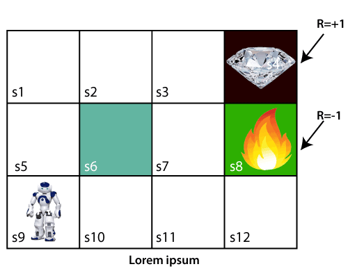
Example problem
- In the above problem, the agent is at s9 and it have to get to s4 for the diamond.
- The agent can move in four directions: up, down, left, and right.
- If it reach s4 (diamond), then it will get a reward of +1.
- If it reach s8 (fire), then it will get a reward of -1.
- The agent can take any path to reach the diamond, but it needs to make it in minimum steps.
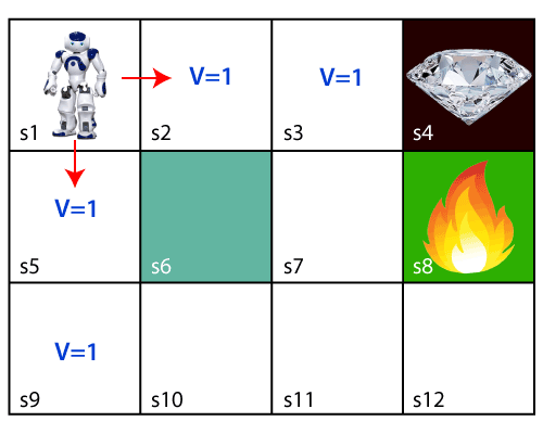
- Initally, the agent will explore the enviroment and try to reach the diamond. As soon as it reachs the diamond, it will backtrace its step back and mark values of all states which leads towards the goal as V = 1.

Result without Bellman
- But, if we change the start position, the agent can not find the path to the goal. So, we need to use the Bellman equation to solve this problem.
Problem without Bellman
8.2 The Bellman Equation
The Bellman equation is used to calculate the expected long-term return of the state, also known as the value of the state.
The Bellman equation is given below:
V(s) = max[R(s) + γV(s')]- The key-elements used in Bellman equation are:
- The agent perform an action
ain the statesand moves to the next states'. - The agent receives a reward
R(s). V(s): It is the value of the state s.V(s'): It is the value of the next state.γ: It is the discount factor, which determines how much the agent cares about rewards in the long-term future or in the short–term future. It has a value between 0 and 1. Lower value encourages short–term rewards while higher value promises long-term reward
- The agent perform an action
With the above example, we start from block s3 (next to the target). Assume discount factor γ = 0.9.
For s3 block. Here V(s’) = 0 because no further state to move. So, the Bellman equation will be:
V(s3) = max[R(s3) + γV(s')] = max[1 + 0.9 * 0] = 1For s2 block. Here V(s’) = 1 because it can move to s3. So, the Bellman equation will be:
V(s2) = max[R(s2) + γV(s')] = max[0 + 0.9 * 1] = 0.9For s1 block. Here V(s’) = 0.9 because it can move to s2. So, the Bellman equation will be:
V(s1) = max[R(s1) + γV(s')] = max[0 + 0.9 * 0.9] = 0.81For s5 block. Here V(s’) = 0.81 because it can move to s1. So, the Bellman equation will be:
V(s5) = max[R(s5) + γV(s')] = max[0 + 0.9 * 0.81] = 0.73For s9 block. Here V(s’) = 0.73 because it can move to s5. So, the Bellman equation will be:
V(s9) = max[R(s9) + γV(s')] = max[0 + 0.9 * 0.73] = 0.66s9 block is also the start block of agent.
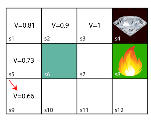
Result using Bellman equation- Now we move to s7 block, here the agent have 3 options:
- UP to s3
- LEFT to s8 (fire)
- DOWN to s11
- Can not move left to s6 because it is a wall.
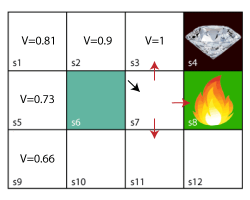
s7 blockThe
maxin Bellman equation denote the most optimal path among all posible action that agent can take at a given state. Among all actions available, the maximum value for that state is the UP action. So, the Bellman equation will be:V(s7) = max[R(s7) + γV(s')] = max[0 + 0.9 * 1] = 0.9Continue the process, we got the final result. The agent will take the path with maximum value by following the increasing value of the states based on the Bellman equation.

Final result
The above Bellman equation maybe cause some confusion for the agent because it only consider the immediate reward. So, we need to use the Bellman Optimality Equation.
V(s) = max_{a}(R(s, a) + γ\sum_{s'}P(s,a,s')V(s'))
Where $P(s,a,s')$ is the probability of transitioning from state s to s’ with action a.
9. Markov Decision Process
9.1 What is Markov Decision Process?
Markov decision process (MDP) is a control process that provides a mathematical framework for modeling decision making in situations where
outcomes are partly random and partly under the controlof a decision maker.MDP is used to describe the environment for the RL, and almost all the RL problem can be formalized using MDP.
MDP contains a tuple of 5 elements $
(S, A, P, R, \gamma)$ where:- S is a set of states (typpically finite)
- A is a set of actions (typpically finite)s
- P is a transition probability matrix. In which $
P(s, s', a) = P(s_{t+1} = s' | s_t = s, a_t = a)$ is the probability of transitioning from state s to s’ with action a - $
R(s, s', a) \in \mathbb{R}$ is the immediate reward after going from state s to s’ with action a. - $
\gamma$ is the discount factor, which determines how much the agent cares about rewards in the long-term future or in the short–term future. It has a value between 0 and 1. Lower value encourages short–term rewards while higher value promises long-term reward.
The agent moves from state to state by observing the environment, taking actions, and receiving rewards at every step. The rewards could be represented as $R_t, R_{t+1}, R_{t+2},…+R_{t+n-1}$ at every time-step t and the agent may achieve its final goal in the n-th step.
Now, we have $G_t$ is the total discounted reward from time-step t, opposite to the total reward $R_t$ which is an immediate return.
G_t=\sum_{k=0}^{\infty}\gamma^kR_{t+k} = R_t+\gamma R_{t+1}+\gamma^2R_{t+2}+\gamma^3R_{t+3}+…
$V^\pi(s)$ is the “state” value function of an MDP (Markov Decision Process). It’s the expected return starting from state s, and then following policy π.
V^\pi(s) = E_{\pi} \{G_t \vert s_t = s\}
$Q^\pi(s, a)$ is the “state action” value function, also known as the quality function. It is the expected return starting from state s, taking action a, and then following policy π. It’s focusing on the particular action at the particular state.
Q^\pi(s, a) = E_\pi \{G_t | s_t = s, a_t = a\}
The relationship between $V^\pi(s)$ and $Q^\pi(s, a)$ is:
V^\pi(s) = \sum_{a ∈ A} \pi (a|s) * Q^\pi(s,a)
You sum every state action-value multiplied by the probability of taking that action (given by the policy $\pi(a|s)$) to get the state value. If you think of the grid world example, you multiply the probability of (up/down/right/left) with the one step ahead of the state value of (up/down/right/left).
Markov Decision Process
9.2 Markov Property
Markov Property define that “If the agent is present in the current state S1, performs an action a1 and move to the state s2, then the state transition from s1 to s2
only depends on the current state and future actionandstates do not depend on past actions, rewards, or states.”In other words, the next state depends only on the current state and action, not on the sequence of events that preceded it. Hence, MDP is an RL problem that satisfies the Markov property.
Mathematically, the Markov property is defined as:
P[S(t+1) | S(t)] = P[S(t+1) | S(t), S(t-1), S(t-2), ... , S(0)] = P[S(t+1) | S(t)]For example in a Chess game, the players only focus on the current state and do not need to remember past actions or states.
The Markov property allows MDP problems to be fully characterized by the transition function between states rather than the full history which means that at any point, we have all the information we need to make decisions based just on the current state. The past is irrelevant for determining the next action.
10. Reinforcement Learning Algorithms
10.1 Q-Learning
10.1.1 What is Q-Learning?
Q-learning is a reinforcement learning technique used by agents to learn what actions to take under what cases. It learns the value function
Q(S, a), which meanshow good to take action "a" at a particular state "s".The below flowchart explains the working of Q-learning:
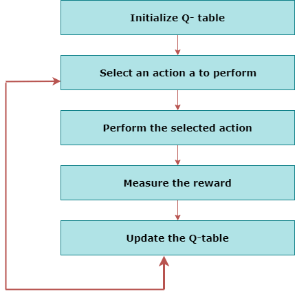
Q-Learning flowchart
10.1.2 An example
- Let’s say that a robot has to cross a maze and reach the end point.
- There are mines, and the robot can only move one step at a time.
- If the robot steps onto a mine, the robot is dead.
- The robot has to reach the end point in the shortest time possible.
- The scoring/reward system is as below:
- The robot loses 1 point at each step. So that the robot have to take the shortest path and reaches the goal as fast as possible.
- If the robot steps on a mine, the point loss is 100 and the game ends.
- If the robot gets power ⚡️, it gains 1 point.
- If the robot reaches the end goal, the robot gets 100 points.
- The problem is how do we train a robot to reach the end goal with the shortest path without stepping on a mine?
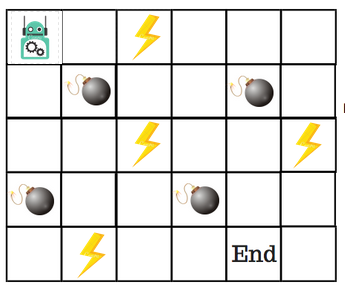
Example problem
10.1.3 Q-Table
- Basically, the Q-table is a look-up matrix where we have a row for each state and a column for each action. Each Q-table cell is a score which will be the maximum expected future reward that the robot will get if it takes that action at that state. This is an iterative process, as we need to improve the Q-Table at each iteration.

Q-table
- For the above example:
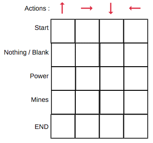
Q-table for above problem
10.1.4 The Q-Learning algorithm
- The main process of Q-Learning algorithmn:
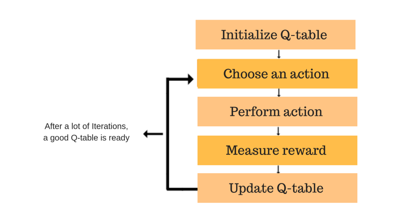
Main process of Q-Learning algorithmn
- Step 1: Initialize the Q-table with zeros.
- There are n columns, where n is number of actions. There are m rows, where m is number of states.
- We will initialise the values at 0.
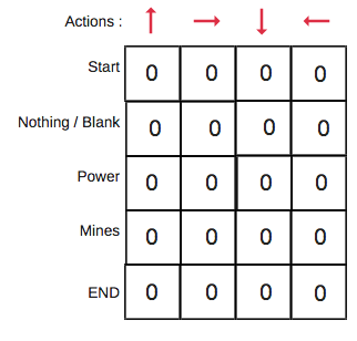
Initialize the Q-table with zeros
- Steps 2 and 3: choose and perform an action.
This combination of steps is done for an undefined amount of time. This means that this step runs until the time we stop the training, or the training loop stops as defined in the code.
In each step, we choose an action using the
epsilon-greedy policy. This means we will decide to choose the action with the highest Q-value for the current state, or a random action.- Epsilon-greedy policy based on epsilon value (in range 0 to 1).
- First, we choose a random number between 0 and 1.
- If the random number is less than epsilon, we choose a random action.
- If the random number is greater than epsilon, we choose the action with the highest Q-value for the current state.
- So, if the epsilon value is 0.1, then 10% of the time, we will choose a random action, and 90% of the time, we will choose the action with the highest Q-value for the current state.
- It is a trade-off between exploration and exploitation. With higher epsilon values, we explore more, and with lower epsilon values, we exploit more.
- In practice, we start with a higher epsilon value and then gradually decrease it as the training progresses. This is because we want to explore more in the beginning and exploit more towards the end of the training.
- Steps 4 and 5: evaluate.
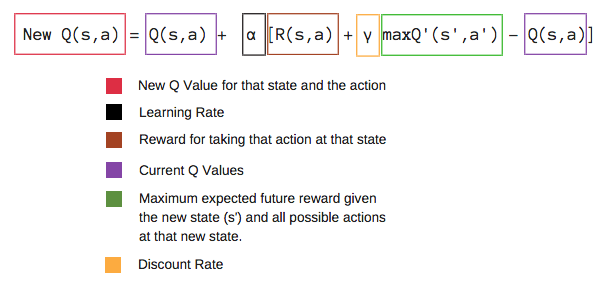
- Now we have taken an action and observed an outcome and reward. We need to update the function Q(s,a).
Q-table update formula- Discount rate is a value between 0 and 1. It is used to balance immediate and future reward. Very low discount consider immediate reward while high discount care future reward. The true value of the discount factor is application dependent but the optimal value lies between 0.2 to 0.8.
- We will repeat this again and again until the learning is stopped. In this way the Q-Table will be updated.
10.2 Deep Q Network (DQN)
As the name suggests, DQN is a Q-learning using Neural networks.
The limitation of Q-learning is that if the state is too large, it will take a lot of space to store the Q-table and slow down the learning time because during the learning process the Q-table is accessed continuously.
To solve such an issue, we can use a DQN algorithm. Where, instead of defining a Q-table, neural network approximates the Q-values for each action and state.

Q-Learning vs Deep Q-Learning
11. Future of Reinforcement Learning
- There are many potential future applications of reinforcement learning:
- Autonomous vehicles: Using RL for perception, navigation, decision making and end-to-end driving of self-driving cars without human intervention.
- Robotics: Developing intelligent robots that can perform complex physical tasks like assembly, manipulation, locomotion etc. using RL.
- Game AI: Creating game agents and bots that can achieve expert level skills across a variety of games.
- …
12. References
- TBD